Chapter 2

2 Emotion Recognition Basics

This chapter gives an introduction to the state of the art in emotion recognition theory. The present system stems from research inputs from varied sources due to papers and hypothesis presented by psychologists, linguists, and research in the field of neural networks and other classifiers.

Section 2.1 gives a brief psychological perspective called the Activation-Evaluation hypothesis on how emotions can be modeled using a two dimensional space where one dimension represents the strength of the emotion and the other represents how positive or negative the emotion is.

Section 2.2 describes the classifier used in this thesis, which takes as input the features extracted according to the activation – evaluation hypothesis from an utterance and outputs what it thinks as the emotion expressed by the speaker.

2.1 Activation – Evaluation Space Theory

From the current psychological hypothesis, activation-evaluation space represents emotional states in terms of two dimensions. Activation measures how dynamic the emotional state is. For instance, exhilaration involves a very high level of activation; boredom involves a really low one.

Evaluation is a global measure of the positive or negative feeling associated with the emotional state. For instance happiness involves a very positive evaluation; Despair involves a very negative one. The circumference is defined by states that are at the limit of emotional intensity. These are equidistant from an emotionally neutral point i.e. they define a circle, with alert neutrality at the center.

[2]Figure 2‑1 FeelTrace Display as extracted from the publication [Rod 00]

2.1.1 Prosodic Features

Emotion is an integral component of human speech, and prosody is the principle conveyer of the speaker’s state and hence is significant in recovering information that is fundamental to communication.

The acoustic prosodic features are signal-based attributes that usually span over speech units that are larger than phonemes (syllables, words, turns, etc). Within this group two types can be further distinguished:

· Basic prosodic features are extracted from the pure signal without any explicit segmentation into prosodic units. These features are not normally used directly for prosodic classification; instead, they are the basis to calculate more complex prosodic features.

· Structured prosodic features can be seen as variations of basic prosodic attributes over time. Consequently, they are computed over a larger speech unit. Structured prosodic features can derive from the prosodic basic features or can be based on segmental information provided e.g. from the output of a work recognizer.

2.1.1.1 Energy as a prosodic feature for emotion detection

Energy is the acoustic correlated of loudness. In terms of global statistics, energy is proved to be higher in emotions whose activation is also high. On the contrary, low energy levels of energy are found in emotional states with a low activation value.

2.1.1.2 Pitch as a prosodic feature for emotion detection

The acoustic correlate of pitch is the fundamental frequency or F0. Fundamental frequency is considered to be one of the most important attributes in emotion expression and detection (s. [Mon02, Abe01]). From the pitch contour of one utterance we extract the mean, maximum, minimum, variance and standard deviation among other features.

2.1.2 Voice Quality Features

Till date, abundant research in the field relating Prosody has been conducted. However due to conclusions derived from previous experiments, it can be evinced that Prosody cannot independently exist as the sole basis for an effective classification of emotions. From the hypothesis of Activation-Evaluation space theory it is further hypothesized that the acoustic correlate of the activation level is Prosody. 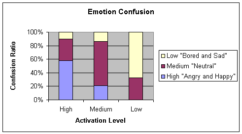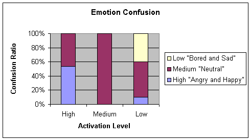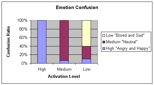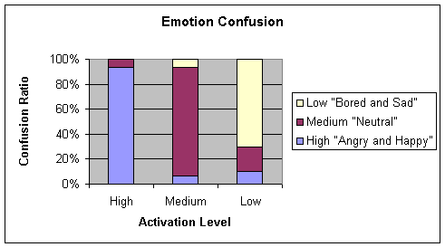This can be proven by the fact that during prosodic experiments, the confusion between emotions such as angry and happy or bored and sad was very high. From Figure 1, it is clearly discernible that angry and happy are having similar values on the activation axis.

From section 2.1, it is clear that there must be another contributing factor to further the differentiation between some emotions. It has been further hypothesized that this other factor, the acoustic correlate of the Evaluation dimension is Voice Quality.

2.2 Neural Network Classifiers

2.2.1 Introduction

In the real world we are confronted with so many systems, which cannot be possibly modeled by a simple series of mathematical equations. These systems do not have a clear-cut decision rule although it is easily conceivable that a relationship must exist between the input and output of the system. Examples of these non-determiNISTic systems range from weather prediction, voice recognition and face recognition systems. 1Wall Street has always looked for methods or systems to find relationships between price movements and economic indicators in the marketplace.

The application of neural networks in these non-determiNISTic systems has met with considerable success and it has shown that they can best model these unknown and abstract functions.

Figure 2‑2 Schema of a non-determinate system

The present application of emotion recognition is a typical example of a non-determiNISTic system wherein an unknown relationship exists between prosodic and voice quality features (input) and emotions (output). We use the artificial neural network to bridge the gap between the prosodic and quality features and emotions.

2.2.2 Definition

An artificial neural network (ANN) is an information-processing paradigm inspired by the way the densely interconnected, parallel structure of the mammalian brain processes information. Artificial neural networks are collections of mathematical models that emulate some of the observed properties of biological nervous systems and draw on the analogies of adaptive biological learning.

The artificial neuron has two modes of operation: the training mode and the using (testing) mode. In the training mode, the neuron can be trained to fire (or not), for particular input patterns. In the using mode, when a taught input pattern is detected at the input, its associated output becomes the current output. If the input pattern does not belong in the taught list of input patterns, the firing rule is used to determine whether to fire or not. [San02]

A neural network is characterized by its particular:

· Architecture: The pattern of connections between the neurons.

· Learning Algorithm: The method used to determine the weights on the connections.

· Activation function: The method used to evaluate the output of the neural network. The most common activation functions are step, ramp, sigmoid and Gaussian function.

2.2.3 Learning Algorithms

The NN models used in this thesis are the Backpropagation Networks including Vanilla Backpropagation and Backpropagation with Chunkwise update and resilient Backpropagation. The description of the following passages has been extracted from the Stuttgart Neural network simulator manual.

2.2.3.1 Backpropagation learning algorithm.

The basic idea of Backpropagation learning algorithm, is the repeated application of the chain rule to compute the influence of each weight in the network with respect to an arbitrary error function E:

(2.1)

Where

w_ij= weight from neuron j to neuron i.

a_i = activation value.

net_i = weighted sum of the inputs of neuron i.

Once the partial derivative of each weight is known, the aim of minimizing the error function is achieved by performing a simple gradient descent:

(2.2)

Where,

η = learning rate.

The user selects learning rate parameter and, as it can be deduced from equation 2.2, it plays an important role in the convergence of the network in terms of success and speed. For the experiments in the following chapters the most commonly used parameters are selected.

The Backpropagation weight update rule, also called generalized delta-rule, for the SNNS software reads as follows:

Text Box: if unit j is an output unit

if unit j is a hidden unit (2.3)

(2.4)

Where

η = learning factor (a constant).

δ_j = error (difference between the real output and the teaching input) of unit j.

o_i = output of the preceding unit i.

t_j= teaching input of unit j.

i = index of a predecessor to the current unit j with link w_ij form I to j.

j = index of the current unit.

k = index of a successor to the current unit j with link w_jk from j to k.

There are several Backpropagation algorithms supplied. The following research makes use of three of the common algorithms. These are as follows

2.2.3.2 Vanilla Backpropagation / Standard Backpropagation

Vanilla Backpropagation corresponds to the standard Backpropagation learning algorithm described above. It is the most common learning algorithm. In SNNS, one may either set the number of training cycles in advance or train the network until it has reached a predefined error on the training set. In order to execute this algorithm, the following learning parameters are required by the learning function that is already built into SNNS.

η: Learning rate specifies the step width of the gradient descent. Typical values of η are 0.1 …1. Some small examples actually train even faster with values above 1, like 2.0.

d_max_: the maximum difference between a teaching value t_j and an output o_j of an output unit which is tolerated, i.e. which is propagated back as d_j=0. If values above 0.9 should be regarded as 1 and values below 0.1 as 0, then d_maxshould be set to 0.1. This prevents over training of the network. Typical values of are 0, 0.1 or 0.2.

2.2.3.3 Backpropagation with Chunkwise update

There is a form of Backpropagation that comes in between the online and batch versions of the algorithm with regards to updating the weights. The online version is the one described before (vanilla Backpropagation). The batch version has a similar formula as vanilla Backpropagation but, while in Vanilla Backpropagation an update step is performed after each single pattern, in Batch Backpropagation all weight changes are summed over a full presentation of all training patterns (one epoch). Only then, an update with the accumulated weight changes is performed.

Here, a Chunk is defined as the number of patterns to be presented to the network before making any alterations to the weights. This version is very useful for training cases with very large training sets, where batch update would take too long to converge and online update would be too unstable.

Besides parameters required in Vanilla Backpropagation, this algorithm needs to fix the Chunk size N, defined as the number of patterns to be presented during training before an update of the weights with the accumulated error will take place. Based on this definition, Backpropagation with Chunkwise update can also be seen as a mixture between Standard Backpropagation (N =1) and Batch Backpropagation (N =number of patterns in the file) For the experiments carried out in this thesis, which make use of this learning algorithm, the Chunk size is set to 50 patterns.

2.2.3.4 RPROP learning algorithm.

Rprop stands for “Resilient back propagation” and is a local adaptive learning scheme, performing supervised batch learning in multi-layer perceptrons.

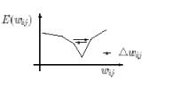
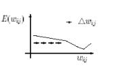
The choice of the learning rate η for the Backpropagation algorithm in equation 2.3, which scales the derivative, has an important effect on the time needed until convergence is reached. If it is set too small, too many steps are needed to reach an acceptable solution; on the contrary a large learning rate will possibly lead to oscillation, preventing the error to fall bellow a certain value. Figure 2.3 shows both phenomena. In case (a), long convergence times are required, and in the (b) case, an oscillation can be seen in the proximity of local minima.

(a) (b)

Figure 2‑3 Error functions for the case of (a) a small learning rate and (b) a large learning rate.[San02]

The basic principle of Rprop is to eliminate the harmful influence of the size of the partial derivative on the weight step. This algorithm considers the local topology of the error function to change its behavior. As a consequence, only the sign of the derivative is considered to indicate the direction of the weight update. The size of the weight change is exclusively determined by a weight-specific, so-called 'update-value' .

Text Box: if
if
else (2.5)

Where

= Summed gradient information over all patterns of the pattern set.

The basic idea for the improvement realized by the Rprop algorithm was to achieve some more information about the topology of the error function so that the weight-update can be done more appropriately. Each ‘update-value’ evolves during the learning process according to its local sight of the error function E. Therefore, the second step of Rprop learning is to determine the new update-values. This is based on a sign-dependent adaptation process:

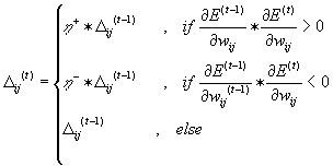
(2.6)

where 0 < η^-< 1 < η⁺

Note that the update-value is not influenced by the magnitude of the derivatives, but only by the behavior of the sign of two succeeding derivatives. Every time the partial derivative of the corresponding weight changes its sign, which indicates that the last update was too big and the algorithm has jumped over a local minimum (figure 6.5a), the update-value is decreased by the factor η^-. If the derivative retains its sign, the update-value is slightly increased in order to accelerate convergence in shallow regions.

Chapter 3

3 Voice Quality Features

„Voice quality is the characteristic auditory coloring of an individual's voice, derived from a variety of laryngeal and supralaryngeal features and running continuously through the individual's speech. The natural and distinctive tone of speech sounds produced by a particular person yields a particular voice.“

Trask (1996:381) [Tra96]

3.1 Introduction

The following passages, which have been extracted from [Mar97] [San02], are first presented to give a brief understanding of the relation between Voice quality features and emotions.

The source-filter theory of speech production hypothesizes that an acoustic speech signal can be seen as a source signal (the glottal source, or noise generated at a constriction in the vocal tract), filtered with the resonance in the cavities of the vocal tract downstream from the glottis or the constriction. Figure 3.6 shows a schema of this process for the case of voiced speech (periodic source signal).

Figure 3‑1

Source filter model of speech production

Voiced sounds consist of fundamental frequency (F0) and its harmonic components produced by vocal cords (vocal folds). But not only the source participates in the speech generation process, also the vocal tract, which acts as a filter (see figure 3), modifies this excitation signal causing formant (pole) and sometimes anti-formant (zero) frequencies [Wit82]. Human perceptual system translates patterns of formant frequencies into specific vowels. Each formant frequency has also amplitude and bandwidth and it may be sometimes difficult to define some of these parameters correctly. The fundamental frequency and formant frequencies are probably the most important concepts in speech processing in general.

With purely unvoiced sounds, there is no fundamental frequency in the excitation signal and therefore no harmonic structure either, and the excitation can be considered as white noise. The airflow is forced through a vocal tract constriction, which can occur in several places between glottis and mouth.

3.2 Relationship between formant characteristics and vowels

To bring the reader to a closer understanding of the relationship between formant characteristics and emotions An extract from Alison Tickle highlighting “To what extent vocalization of emotion is due to psycho-biological response mechanisms and is therefore quasi-universal and to what extent it is due to social convention” will be summarized. The experiment has been conducted with regards to emotion vocalization and recognition, of English and Japanese speakers.

This will be followed by the methodology behind practical implementation of conclusions derived from this paper. For this a slightly deeper understanding of vowels as a function of formants will be needed. This is followed by a brief explanation of the algorithm to detect [a] and [I] regions.

3.2.1 Alison Tickle’s Experiment

A summary of the psychological study conducted by Alison Tickle[Tik00] and its conclusions are presented. The study used non-sense utterances, phonotactically possible in both languages. These permit more cross-language consistency, avoid problems with translation and give no verbal cues. In the present study, non-sense utterances were composed allowing the influence of vowel quality to be highlighted as well as to be compared cross-culturally. Only hypotheses relevant to my thesis and based on previous research were made in relation to the decoding experiment and are explained as follows:

Happy will be least accurately decoded when it is encoded on the utterance containing [a] vowel quality compared to [i] or [u] Bezooijen [Bez84] suggests that happy may be easy to detect on [i] saying that extra lip spreading due, for example to smiling, is easier to detect in unrounded vowels. This study attempts to investigate this further by controlling for vowel quality on non-sense utterances tested on native speakers of unrelated languages.
Angry will be most accurately decoded when encoded on [u] and least accurately decoded on [i]. This hypothesis is based on research by Ohala [Oha84] suggesting that the technique of vocal tract lengthening, thereby signaling a larger sound source, is used by certain animals, when expressing anger or aggression and since [u] necessitates a lengthening of the vocal tract, it is a more likely to be used sound symbolically, to suggest aggression or anger.

3.2.1.1 Encoding Experiment

8 Japanese and 8 English female university students aged between 18 and 35 encoded the data based on visual aids consisting of eight quasi-universally recognized facial expression photographs. The reason for this approach is twofold in that it focuses attention upon emotions to be considered primarily via a visual stimulus, which is common to both language groups and concentrating on the photograph and imitating the facial expressions was found to be a useful stimulus.

3.2.1.2 Data Decoding Experiment

Data from the three most reliable speakers of each language was used in a forced judgment-decoding test. The total number of items presented to decoders included 90 items (3 speakers x 2 languages x 5 emotions x 3 vowel qualities)

3.2.1.3 Data Decoding Procedure

16 English subjects (12 female and 4 male) and 8 Japanese subjects (4male and 4 female) performed a forced judgement-decoding test on the edited data described above. Judges were offered 5 emotion words in their native language from which to choose a single response.

3.2.1.4 Results

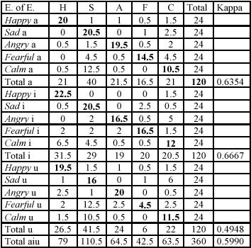
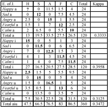
Figure 3‑2, show confusion matrices for English For each Table, the emotions portrayed (English and Japanese) are indicated along the first column and the possible decoding responses are shown across the top row. Abbreviations are used representing English emotion words, the English translations of which are happy (H), sad (S), angry (A), fearful (F) and calm (C).

From the confusion matrices given below it can be evinced that English subjects most accurately decoded emotions encoded by English subjects on [i], then [a] then [u]. Subjects slightly more accurately decode happy on [i] supporting Bezooijen’s suggestion: see the second hypothesis. Interestingly, subjects are also most likely to categorize vocalizations overall as happy when they are encoded on [i]. They are least likely to categorize vocalizations overall as sad on [i] than on [a] or [u]. Angry is least accurately decoded on [i] and vocalizations are least often categorized as angry on [i]: this perhaps lends support to the second hypothesis.

Figure 3‑2: English decoders’ discrimination of emotions encoded by English speakers showing vowel quality, extracted from [Tik00]

From Figure 3‑3, English subjects also scored highest on decoding Japanese vocalizations of emotions on [I], then [a], then [u], again supporting Bezooijen’s suggestion. In addition, where subjects categorize a vocalization as happy this is most likely to be on [i]. They are more likely to decode an emotion as sad on [u] than on [i]. Happy is most often confused with angry on [a] and [i] but with calm on [u], which may be relevant to the fifth hypothesis. However they were most likely to decode vocalizations overall a

Figure 3‑3 English decoders’ discrimination of emotions encoded by Japanese speakers showing vowel quality, extracted from [Tik00]

The conclusions, which can be derived from this experiment and useful for the present thesis, are as follows

· All Emotions are generally, more accurately decoded on [i] as compared to the other vowels [a] and [u].

· The happy emotion in particular is decoded most accurately on [i] and subjects are most likely to categorize vocalizations overall as happy when they are encoded on [i].

· The angry emotion is least likely to be decoded on [i] and vocalizations are least likely to be categorized as angry on the [i] region.

From the above experiment, one can conclude that the vocal effects of possibly quasi-universal psycho-biological response mechanisms may be signaling distinctions between the emotions under consideration here which are enhanced in specific vocal regions (from the conclusion of this experiment, in the [i] region). Also vocal effects were speaker independent since there were 6 speakers in total from which the data was derived. It could be possible that the acoustic properties of the voice signal in this region [i] could be an instrumental aid in distinguishing between emotions. This is the hypothesis we make from the conclusions of [Tik00] and the philosophy behind practical implementation of extraction of the [a] and [i] regions from a voice signal. The next question would be how could one distinguish a [a] or [i] region from the voice signal. This is where the acoustic characteristics of vowels come into picture and for a deeper understanding of formants as a function of the physical characteristics of the voice production system, an extract from [Ven96] is explained below.

3.2.2 Acoustic Characteristics of Vowels

Vowels are characterized by the presence of relatively intense and well-defined formants. First three formants are adequate to perceptually discriminate between all English vowels. Source spectrum for vowels is a complex periodic sound from the larynx. High vowels have higher fundamental frequency or f₀ than low vowels because of the elevation of the larynx.

· The first formant or F₁is primarily determined by the back cavity - the size of the cavity behind the tongue hump. The back cavity is larger for the high vowels than for low vowels because, for high vowels, the tongue is pulled forward and up. A larger cavity results in a low F₁ for high vowels.

· The second formant or F₂ is primarily determined by the front cavity - the cavity in front of the tongue hump. Front vowels have small front cavity and, therefore, lower F₂. Lip rounding results in a larger front cavity and consequently a lower F₂.

· The third formant or F₃ is a function of the entire vocal tract; the degree of coupling between the front and back cavities primarily determines the value of F₃. Low vowels result in greater coupling between the two cavities and therefore, lower F₃.

[i]

High, front

Low F₁

High F₂

High F₃

[u]

High, back

Low F₁

Low F₂

High F₃

Low, front

High F₁

High F₂

Low F₃

[ae]

Low, back

High F₁

Low F₂

Low F₃

[a]

Table 3‑1Vowels as a described by their formant characteristics, extracted from [Ven96]

Hence a difference in the position of the first and second formant (F₁ and F₂), normalized by the first formant position, is used as a value for detecting [a] and [I] phonemes. Very generally, Phoneme [a] has the first and second formant very close, and the first formant position very high, and phoneme [I] the exact opposite i.e. The distance between first and second formant is larger than for other vowels, and the first formant position is very low.

Assuming a selected region from one utterance, the mean of the values (F₂- F₁)/ F₁ is calculated for all the frames in the voiced region. For each utterance the maximum and minimum of the values mean (F₂- F₁), max/min (mean (F₂- F₁)/ F₁) is computed and the corresponding voiced region is labeled as an [a] or [I] respectively. The quality features will be calculated in either of the two, following the previous criteria.

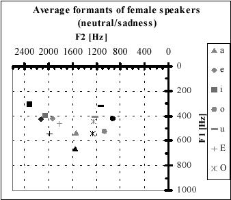
Figure 3‑4. Average formant values for sadness (Grey symbols) compared with neutral (black symbols) of female speakers as extracted from [kie00].

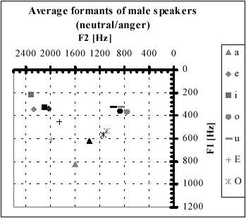
Figure 3‑5. Average formant values for anger (Grey symbols) compared with neutral (black symbols) of male speakers as extracted from [Kie00]

3.2.2.1 Emotions as a function of vowels and formants

Another paper by [Kie00] illustrates the relationship between emotions and formant values (F₁ F₂) of each vowel. It was observed from Figure 3‑4 and Figure 3‑5 that sentences expressing fear, sadness and boredom are characterized by a formant shift towards a centralized position. It simply means that in these emotions there is a minimal tendency towards articulating each vowel. In contrast, the emotions angry and happy have the formant spectrum distributed over a wide region. This indicates that speech is more pronounced and accentuated in these emotions. From the above two papers, it can be concluded that formant features can be used

· To distinguish between voiced regions containing [a] and [i] to extract the best features from these regions for emotion classification. [Tik00]

· As input features for emotion classification. [Kie00]

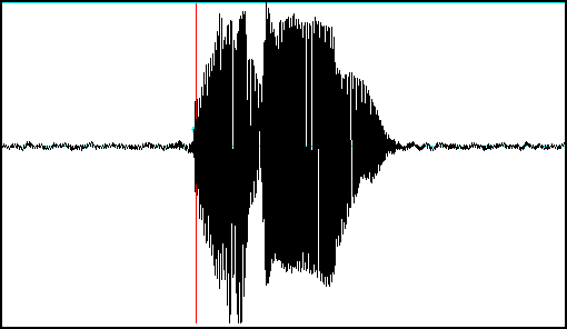
3.2.3 Formants: A visual representation

The speech signal shown below is the visual representation of an utterance extracted from the Sony emotion database in the time and frequency domain. The content of the utterance is the word “Hallo” spoken in German. The following diagrams have been extracted from the PRAAT software.

0 3.45s

Time ‘t’

Figure 3‑6: The command “Hallo” emoted in angry tone

To define the frequencies that are present at any given moment in the speech signal, the Fourier Transformation is used. The result of Fourier analysis is called spectrum. A spectrogram is created by displaying all of the spectra together, envisions how the different frequencies change over time. Figure 3‑7 shows the spectrogram generated from the waveforms of Figure 3.6. The x-axis of the spectrogram shows positive time toward the right, as it did for the waveform, and the y-axis presents frequencies up to 5000 Hertz. The gray scales of the spectrogram represent the importance of the acoustic peaks for a given time frame. The darkest horizontal bars give the highest energy, usually belonging to vowels. These parts are called formants.

0 Time ‘t’ 3.45s

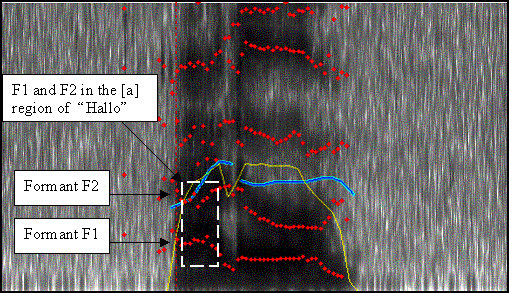
Figure 3‑7 Spectrogram of the above voice utterance “Hallo” indicating the formant frequencies, fundamental frequency.

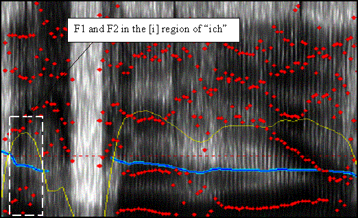
From Figure 3‑7and Figure 3‑8, the dashed boxes display the values of the formant frequencies in the [a] region of “Hallo” and in the [i] region of “Ich” respectively. The horizontal bands in Figure 3‑7 are much closer in this region with a high F₁and low F₂indicating a [a] region. By contrast in Figure 3.8, the horizontal bands are much further apart with a low F₁and high F₂ indicating a [i] region.

1.53s Time ‘t’ 4.78s

Figure 3‑8 Spectrogram of the voice utterance “ich bin hier“

3.2.4 Algorithm Design for calculation of [a] and [i] regions

For every voiced region inside an utterance:

f1temp=Get first formant #first formant freq.

f2temp=Get second formant #second formant freq.

dif=f2temp-f1temp

coc_temp=dif/f1temp

· First formant frequency must not be higher than 1.2KHz

· Second formant frequency must not overpass 2KHz

· 10% tolerance to admit candidates, whose first formant frequency is not maximal but it is compensated by a closer position of the first two formants

if (f1temp>f1max) or ((f1temp/f1max>0.9) and (dif<dif_temp))

The lowest formant ratio is chosen with a 10% tolerance.

To avoid confusion with /u/, candidates whose second formant freq. is lower than 1000 are discarded

if(coc_temp/coc<1.1)or((coc/coc_temp>0.9)and(f2max<1000)){

coc=coc_temp

f1max=f1temp

f2max=f2temp

}

If the region satisfies all the requirements, following parameters are stored:

f1=f1temp # first formant freq.

f2=f2temp # second formant freq.

End for

3.3 List of Quality Features.

This section gives a brief description of the quality features, which have been calculated as per previous research work. The quality features as explained in Section 2.1.2, are responsible for the evaluation/ pleasure dimension of the emotion model in Figure 2‑1. The software used to compute quality features is PRAAT, a freeware program developed by Dr. Paul Boersma and David Weenink, Institute of Phonetic sciences at the University of Amsterdam. The software is a research, publication, and productivity tool for phoneticians.

The quality features can be categorized into the following sections:

1. Harmonicity based features

2. Formant frequency based features

3. Energy based features

4. Spectral tilt related features

Since the features listed below have been results of past research conducted at MMI Lab, Sony International GmbH only a brief explanation of the features is given below. For further extensive reading please refer to [San02].

3.3.1 Calculation of the Mean

This section makes use of two different methods for the calculation of the mean value of a given quality feature within a voiced region:

Mean1: Arithmetic mean of the parameter values over all the frames inside a voiced region.

Where

nframes = number of frames inside a voiced region.

f_i = feature value in the frame i.

Mean2: First, the Mean1 of the parameter within a voiced region is computed. Then, single values of this parameter for every frame are checked and the one, which is closest to the computed Mean1, is considered as the mean (Mean2) of this region. This way, we assume that this value comes from the most representative part inside the voiced region, since the mean is influenced also by voiced region boundaries. It was experimentally checked that the chosen frames normally matches the core of the vowel.

Where

nframes = number of frames inside a voiced region

n = index of the region

f_i = feature value in the frame i

= Mean1 of the feature in region n

From now, they are referred as Mean1 and Mean2 in the subsequent feature calculation description.

3.3.2 Harmonicity based features.

Since harmonic to noise ratio is clearly related to the voice quality, this voice quality attribute has been said to provide valuable information about the speaker’s emotional state (s. [Error! Reference source not found., Alt00]). Harmonic to noise ration estimation can be considered as an acoustic correlate for breathiness and roughness, in agreement with [Alt00]. Therefore, voice quality cues, which help us to infer assumptions about the speaker’s emotional state, can be extracted from this attribute.

There are in total 13 harmonicity-based features, which have, been computed and these are, namely HNR maximum, HNR means, HNR ranges over mean1 and mean2.

3.3.3 Formant frequency based features.

For each analysis window, Praat applies a Gaussian-like window, and computes the LPC coefficients with the algorithm by Burg. The Burg algorithm is a recursive estimator for auto-regressive models, where each step is estimated using the results from the previous step. The implementation of the Burg algorithm is based on the routine memcof and zroots in [Pre93]. This algorithm can initially find formants at very low or high frequencies. From the values obtained for every single frame, some features are computed, which will be used as input for the emotional classification.

In total, 30 formant features have been computed and these are:

1. Formant frequency minimum f2_Mean – f1_Mean for all the voiced regions and means (2 features)

2. Formant frequencies for 3 formants subscripted by their means (6 features)

3. Formant ratios (4 features)

4. Formant bandwidths (9 features)

5. Maximum of a formant in a selected region (3 features)

6. Range of a formant in a selected region (3 features)

7. Standard deviation of a formant in a selected region (3 features)

3.3.4 Energy based features.

The energy is calculated within four different frequency bands in order to decide, whether the band contains mainly harmonics of the fundamental frequency or turbulent noise. Frequency band distribution is taken from a study [Kla97] focused on the perceptual importance of several voice quality parameters. The four frequency bands proposed are:

1. From 0 Hz to F0 Hz (where F0 is the fundamental frequency).

2. From 0 Hz to 1 kHz.

3. From 2.5 kHz to 3.5 kHz

4. From 4 kHz to 5 kHz.

There are in total, 10 energy based features.

3.3.5 Spectral measurements.

There are two classes of spectral based quality features:

1. Open quotient related features.

Open quotient is a spectral measurement whose variations have been associated to changes in the glottal source quality. Hence it would be a useful parameter in order to determine the emotional state of the speaker.

2. Spectral Tilt related features.

From [San02], Spectral Tilt has been also related to glottal source variations. It is one of the major acoustic parameters that reliably differentiate phonation types in many languages, and it can be understood as the degree to which intensity drops off as frequency increases. Spectral tilt can be quantified when comparing the amplitude of the fundamental to that of higher frequency harmonics, e.g. the second harmonic, the harmonic closest to the first formant, or the harmonic closest to the second formant. Spectral tilt is characteristically most steeply positive for creaky vowels and most steeply negative for breathy vowels

Chapter 4

4 Experiments with Prosodic Features

This chapter gives an explanation of the experiments conducted till date. Prosodic features are employed to classify the level of activation. The first series of experiments have been preliminary and the motivation behind conducting these was to get a clearer understanding of the present system, temporal research goals as well as the directions for further research upon which I will be basing the work for this master thesis. The sequence of steps involved whilst performing the experiment is as follows:

4.1 Experiment Sequence

4.1.1 Data preprocessing

Input to the system consists of voice samples from the Sony International GmbH database. These are stored in NIST file format. The first program is used to cut the header of the NIST file. The ‘National Institute of Standards and Technology, USA’ defined the NIST speech header format. Hence input to the data pre processing sub-system is the emotional recording in NIST format and the output is the same file without header and with the bytes of each sample swapped.

4.1.2 Feature Calculation

Compute_basismerkmale.c is the basic prosody module of the VERBMOBIL project. It extracts the fundamental frequency contour, energy contour and voice/unvoiced decision of each frame from an input speech file. These contours are used by another program written by Rocio Santos for calculating prosodic features as well as calculating voiced and unvoiced regions. PRAAT scripts for calculating voice quality features will later on utilize these regions. The output of this sub system is a feature file, which consists of a series of numbers representing prosodic features where each line represents each utterance.

4.1.3 Normalization

The feature files then serve as an input to two program files, which are used to calculate statistics for each feature like absolute maximum, mean. These are normalized between values of –1 to 1. After normalization, patterns files are created for training, evaluating and testing the network. These files are passed through a Perl program, which inserts SNNS pattern header for compatibility. These Perl programs have been designed and programmed by Dr. Vicky Lam, scientist at the MMI lab, Sony International GmbH.

4.1.4 Testing and Training

The software utilized to train and test the neural network classifiers is the Stuttgart Neural Network Simulator (SNNS 4.2), developed at University of Stuttgart and maintained at University of Tübingen. SNNS offers a batchman program, which serves basically an additional interface to the kernel that allows easy background execution. These batchman scripts can be embedded in Perl programs, which in turn are executed for training and testing different network topologies.

Figure 4‑1 Block Diagram schema of the Emotion recognition system

4.2 Experiment Template

In order to provide this document with all the valuable information concerning the experiment conditions, the same schema is used for the description of each one of the experiment series. This schema contains the following aspects, further information about them can be found in the pointed sections of this document.

4.2.1 Objective

· Set of patterns: It specifies whether it is speaker dependent or independent case and which and how many patterns are used for training and/or testing.

· Input features: Mention of the input features utilized according to their description. When more than one set is tried, all of them are here enumerated.

· Output features: The intention of the experiment, which emotions or groups of emotions are to be differentiated. When more than one NN output configuration is tried, all of them are here enumerated.

4.2.2 Conditions

· Normalization: Normalization is made to give the neural network similar range values in all the input nodes, regardless their magnitude. Here, it is specified which divisor vector has been used in this task.

· Neural network (NN) configuration: Information about the neural networks tried; number of layers and hidden nodes, activation function and learning algorithm employed. All the configurations tried are here mentioned, despite only the most significant results are commented. For a clearer understanding of the topologies used in the thesis please refer to Section 2.2.

· Analysis function: Once we get the neural network outcomes, we need a decision rule to determine the emotion of the input sentence.

4.2.3 Results and conclusions

· Confusion matrix, considerations and conclusions are presented. Despite an experiment can try many different configurations, only the optimal case is usually analyzed and presented here.

4.3 Preliminary Experiments

4.3.1 Cross Validation vs. 70-15-15

A couple of experiments were performed to illustrate the difference between cross-validation and the 70-15-15 test. These are two different neural network training and testing procedures and the result of both the procedures is an indication of which of these two procedures is suitable for the present database.

a) The 70-15-15 procedure involves around seventy percent of the patterns for training and the remaining for evaluating and testing of the NN. This method has inherent drawbacks in the present system, since for the results of this method to be statistically correct; the number of patterns must be large in number.

b) The cross-validation procedure involves the following steps. A single pattern is extracted from the pattern set and the neural network is trained with the remaining patterns. Finally the network is tested with this extracted pattern. This process is repeated iteratively till the NN is tested for each and every pattern in the system. It should be noted that the NN is initialized for each iteration. The results of this method are an average of the results for each iteration. From a statistical standpoint, this is more accurate than the 70-15-15 case, if the amount of data is not sufficient which is true in the present case since the emotion database does not contain a large data set.

c) Testing with a noisy microphone: The following experiment has been used to test the system with data extracted from a standard m3 SONY microphone. Prior to this, all experiments were conducted using a high quality C38B condenser microphone. This experiment was performed keeping in mind, the possibility of demonstrations for future AIBO prototypes conducted with a standard microphone and the testing of the robustness of the Neural Network with data mixed with noise.

Ø Objective

· Set Of Patterns

Speaker dependent case, Raquel Tato consisting of 814 patterns. Neutrals are always duplicated, since on the activation level we are classifying 5 emotions into 3 categories of high (angry and happy), low (sad and bored) and base (neutral). The network must be trained with equal number of patterns from all three levels, as a result of which the neutrals are duplicated.

· Input features:

P1.0-P1.36 36 prosodic features consisting of energy and fundamental frequency, fundamental frequency derivative contour.

· Output features

Happy and Angry (1 0 0), Neutral (0 1 0), Sad and Bored (0 0 1)

Ø Conditions

· Normalization

Normalized by maximum of all the patterns in the training set

· Neural network (NN) configuration

No hidden layer; logistic activation function; Standard Backpropagation and Backpropagation with Chunkwise update learning algorithms with multiple step training.

Ø Results and conclusions

The resulting tables indicate the confusion matrix format of the network results. Confusion among emotions could yield valuable information regarding insight into new relational hypothesis between the emotions. In confusion tables, rows represent the emotions expressed by the speaker and columns are the neural network decision and the values represent the guess percentages. Hence the left diagonal of the matrix must contain elements with values 100 for a perfect classifier.

	Happy/Angry	Neutral	Bored/Sad
Happy/Angry	95.65	4.35	0.00
Neutral	16.67	35.00	48.33
Bored/sad	2.17	10.87	86.96

Table 4‑1 Confusion matrix of 4.3.1 a (70-15-15) for the Chunk learning algorithm

Average = 69.07

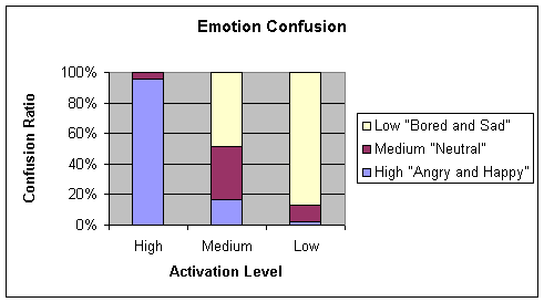
Chart 4‑1 Graphical representation of Table 4-1

Comparing tables Table 4‑1 (70-15-15) and Table 4‑2 (cross-validation), it can be inferred that the range of values along the diagonal in the latter case is less extreme. The average balance of emotions is significantly higher showing a six percent improvement.

	Happy/Angry	Neutral	Bored/Sad
Happy/Angry	85.76	13.65	0.59
Neutral	9.76	76.83	13.41
Bored/sad	1.92	38.66	59.42

Table 4‑2 Confusion matrix of 4.3.1 b (cross-validation) for the Stdbp learning algorithm

Average = 74.33

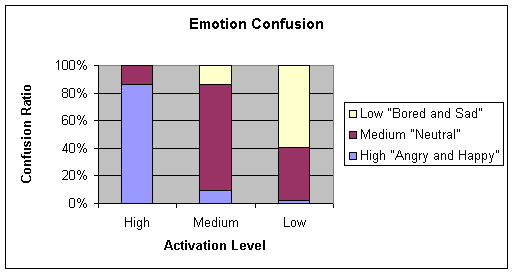
Chart 4‑2 Graphical representation of Table 4-2

Comparing Table 4‑2 and Table 4‑3, the conditions for testing the NNs were identical with the sole exception of the microphones used during the emotion recordings. C38 condenser microphone for Table 4‑2 and M3 standard Sony microphone for Table 4‑3. Hence it can be inferred that the NN is robust when data from a low quality microphone (in the case of the M3 standard microphone) is introduced into the network

	Happy/Angry	Neutral	Bored/Sad
Happy/Angry	90.50	9.50	0.00
Neutral	11.59	73.17	15.24
Bored/sad	4.15	37.70	58.15

Table 4‑3 Confusion Matrix of 4.3.1c (Low quality Microphone)

Average = 74.33

Chart 4‑3 Graphical representation of Table 4-3

4.3.2 Changing the Input Data

A background history of the emotions database must be explained for the basis behind the following two experiments. It was concluded from previous research that during the emotion recording was not accurate since the neutrals contained emotional content. This was because of the recording mechanism wherein neutrals would have been recorded between extreme emotions. From the speaker’s perspective, a neutral emotion would be difficult to elicit in such a situation. These sets of recordings were called stories. It was then decided to record the neutrals separately as read text. These set of recordings are called commands.

Ø Objective

CASE A Speaker dependent case, Raquel Tato stories and commands consisting of 814 patterns.

CASE B Raquel Tato commands

· Input features:

P1.0-P1.37 37 prosodic features consisting of energy and fundamental frequency, fundamental frequency derivative contour and jitter.

· Output features

Happy and Angry (1 0 0), Neutral (0 1 0), Sad and Bored (0 0 1)

Ø Conditions

· Normalized by maximum of all the patterns in the training set

· Hidden layers HD1=10 HD2=5; logistic activation function; Standard Backpropagation and Backpropagation with Chunkwise update learning algorithms with multiple step training.

· WTA (Winner Takes All) Analysis function.

Ø Results and conclusions

Neutrals seem to be more corrupted or confused since the test uses the combination of commands and stories. Bored/sad and neutral are confused more often than angry, which might indicate that bored sad and neutral might lie closer to each other on the activation plane as compared to angry and neutral. This is my hypothesis for the moment from this experiment.

	Happy/Angry	Neutral	Bored/Sad
Happy/Angry	92.28	6.23	1.48
Neutral	17.86	43.45	38.69
Bored/sad	2.24	13.42	84.35

Table 4‑4 Confusion matrix of 4.3.2a (stories and commands) for the Chunk learning algorithm

Average = 73.123734

Chart 4‑4 Graphical representation of Table 4-4

While comparing Table 4‑4 and Table 4‑5, it can be inferred that the hypothesis suggesting that emotional content was present in Stories recordings is true since the confusion on the Neutral row is much higher in Table 4‑4.

	Happy/Angry	Neutral	Bored/Sad
Happy/Angry	85.20	14.80	0.00
Neutral	8.16	75.51	16.33
Bored/sad	1.53	21.43	77.04

Table 4‑5 Confusion matrix of 4.3.2b (Commands) for the Stdbp learning algorithm

Average = 79.251701

Chart 4‑5 Graphical representation of Table 4-5

4.4 Prosodic Experiments with Thomas’ Data

The following experiments are derivatives from the experiment of page 207 in Rocio’s thesis. The objectives of these experiments is to first train and test the neural network with the raw data (.NIST files) and later on make comparative results with data mixed with noise (.e000.m3.NIST). The organization of the experiments is based on the number of patterns introduced to the NN. In other words, I have divided this section into 3 parts.

· The first case is making use of all the data from Thomas, including stories and commands. (.NIST files)

· The second case is making use of all data from stories and only neutral emotions from commands. (.NIST files)

· The third case is making use of all data from Thomas stories and only neutral emotions from commands mixed with noise. (.e000.m3.NIST)

I have abbreviated the conventional way of dividing the pattern files into seventy percent, fifteen percent and fifteen percent for training, evaluation and testing as the 70-15-15 method.

4.4.1 Case 1 Thomas stories and commands

Ø Objective

· Speaker dependent case, Thomas.

· All patterns from Thomas stories and commands

· Input features

10 Prosodic Features

· Output features

Happy and Angry (1 0 0), Neutral (0 1 0), Sad and Bored (0 0 1)

Ø Conditions

· Normalized by maximum of all the patterns in the training set

· 2 hidden layers HD1=10 HD2=5; logistic activation function;

Ø Results and Conclusions

The experiment conducted did not yield good results. The best one is shown in the Table 4‑6 below:

	Happy/Angry	Neutral	Bored/Sad
Happy/Angry	70.13	22.35	7.52
Neutral	12.22	66.06	21.72
Bored/sad	0.94	19.29	79.76

Table 4‑6 Confusion matrix for Rprop 0.2 50 4 learning algorithm using cross validation algorithm

TOTAL: 71.872

Chart 4‑6 Graphical representation of Table 4-6

Again using 70-15-15 method yielded erroneous results due to lack of sufficient amount of patterns, hence statistics depending on chance of the distribution of the patterns over training evaluating and testing.

The results are shown below:

	Happy/Angry	Neutral	Bored/Sad
Happy/Angry	58.21	31.34	10.45
Neutral	21.13	64	14
Bored/sad	0	32.86	67.14

Table 4‑7 Confusion matrix for Stdbp learning algorithm

Average = 63.46

Chart 4‑7 Graphical representation of Table 4-7

In general, when the whole pattern set consisting of Thomas stories and commands are used, the results are the worst among all three cases. Also Rprop algorithm gave the best results for all the cases.

4.4.2 Case 2 Thomas Stories and only neutral commands

Ø Objective

· Speaker dependent case, Thomas.

· All patterns from Thomas stories and only neutrals from commands

· Input features:

10 Prosodic Features

· Output features

Happy and Angry (1 0 0), Neutral (0 1 0), Sad and Bored (0 0 1)

Ø Conditions

· Normalized by maximum of all the patterns in the training set

· 2 hidden layers HD1=10 HD2=5; logistic activation function;

Ø Results and Conclusions:

a. Cross-Validation Test:

	Happy/Angry	Neutral	Bored/Sad
Happy/Angry	75.86	20.69	3.45
Neutral	13.89	70.14	15.97
Bored/sad	1.65	17.36	80.99

Table 4‑8 Confusion matrix for Rprop 0.5 50 4 learning algorithm

Average = 75.36

Chart 4‑8 Graphical representation of Table 4-8

NN training was performed using Rprop algorithm in the single step mode. The cross-validation test was performed only for Rprop 0.5 50 4, since this was yielding the best results and due to length of computation time for the following experiments, I have made the general assumption that the other networks would not perform much better than this one or average close to this one.

b. 70-15-15 Test

	Happy/Angry	Neutral	Bored/Sad
Happy/Angry	58.21	31.34	10.45
Neutral	21.13	64	14
Bored/sad	0	32.86	67.14

Table 4‑9 Confusion matrix for Rprop 0.3 50 4 learning algorithm

Average = 65.625

Chart 4‑9 Graphical representation of Table 4-9

It will be seen from case 3, that the system when mixed with noise performs better than the system without noise. Please refer to Section 6 Conclusions for an explanation of this phenomenon.

4.4.3 Case 3 Thomas stories and only neutral commands mixed with noise

Ø Objective

· Speaker dependent case, Thomas.

· All patterns from Thomas stories and neutrals from commands with noise

· Input features:

10 Prosodic Features

· Output features

Happy and Angry (1 0 0), Neutral (0 1 0), Sad and Bored (0 0 1)

Ø Conditions

· Normalized by maximum of all the patterns in the training set

· 2 Hidden layers HD1=10 HD2=5; logistic activation function;

Stdbp and Chunk update single step

Rprop single step

Rprop single step with pruning

Ø Conclusions and Results

a. Stdbp and Chunk

The first experiment tried was with Stdbp and Chunk. The results were averaging at around 65%.

	Happy/Angry	Neutral	Bored/Sad
Happy/Angry	53.33	46.67	0.00
Neutral	0.00	100.00	0.00
Bored/sad	10.00	50.00	40.00

Table 4‑10 Confusion matrix for Stdbp learning algorithm

Average = 67.500000

Chart 4‑10 Graphical representation of Table 4-10

b. Rprop using 70-15-15

Then Rprop-learning algorithm was used. The results were a bit extreme indicating a possibility of erroneous statistics. I took a look at the result files and found that an error in the classification of a pattern resulted in a steep 6-7% increase/decrease in the confusion matrix statistics. 2 results are shown below

	Happy/Angry	Neutral	Bored/Sad
Happy/Angry	100.00	0.00	0.00
Neutral	6.67	93.33	0.00
Bored/sad	10.00	30.00	60.00

Table 4‑11 Confusion matrix for Rprop 0.5 50 4 learning algorithm using 70 – 15 – 15

Average = 87.500000

Chart 4‑11 Graphical representation of Table 4-11

	Happy/Angry	Neutral	Bored/Sad
Happy/Angry	93.33	6.67	0.00
Neutral	6.67	86.33	6.67
Bored/sad	10.00	20.00	70.00

Table 4‑12 Confusion matrix for Rprop 0.6 50 4 learning algorithm using 70-15-15

Average = 85.5

Chart 4‑12 Graphical representation of Table 4-12

This indicates that by chance probability a “good” set of patterns was taken for testing, which resulted in these figures.

c. Rprop Using Cross validation

The next step would be to run a cross-validation test to test the authenticity of Table 4‑11. The results of this are shown in the next table and the figures show that although it isn’t too far from Table 4‑11, the results are still good. The best 2 results are as follows

	Happy/Angry	Neutral	Bored/Sad
Happy/Angry	84.52	12.26	3.23
Neutral	12.50	72.92	14.58
Bored/sad	1.65	12.40	85.95

Table 4‑13 Confusion matrix for Rprop 0.5 50 4 learning algorithm with cross validation test

Average = 80.95

Chart 4‑13 Graphical representation of Table 4-13

	Happy/Angry	Neutral	Bored/Sad
Happy/Angry	80.00	16.7	3.3
Neutral	15.28	70.14	14.58
Bored/sad	2.48	9.09	88.43

Table 4‑14 Confusion matrix for Rprop 0.6 50 4 learning algorithm with cross validation test

Average = 79.04

Chart 4‑14 Graphical representation of Table 4-14

d. Pruning (Stdbp 0.1 0.2 ) + Rprop training using 70-15-15

Finally the results for network pruning(Stdbp 0.1 0.2) + Rprop were not too different from the ones presented in Rprop using 70-15-15. The results are as indicated below:

	Happy/Angry	Neutral	Bored/Sad
Happy/Angry	86	13	0
Neutral	6	93	0
Bored/sad	20	20	60

Table 4‑15 Confusion matrix for pruning(Stdbp 0.1 0.2 ) and Rprop 0.6 50 4 learning algorithm with cross validation test

Average = 82.5

Chart 4‑15 Graphical representation of Table 4-15

4.5 Summary of Experiment Results for Thomas

CASE 1

All patterns with no noise

CASE 2

Stories and neutral commands with no noise

CASE 3

Stories and neutral commands with noise

Cross validation using Rprop

71.87

75.36

80.95

70-15-15 Stdbp andchunk

67.500000

70-15-15 Rprop

63.46

65.625

87.5

70-15-15 Rprop + pruning

82.5

Figure 4‑2 Summary of the prosodic experiments conducted on the speaker Thomas

Please note regarding the value 65.625 in the table corresponding to “70-15-15 Rprop” and “stories and neutral commands with no noise”. This value should have been at least close to the results of previous research work conducted at Sony but this was not so. Hence I performed another test, and this time I did not use the randomizing function which is normally used to divide the patterns into train-evaluation-test, but I gave a new format to the entire pattern set in the way the patterns are ordered while training. The original goal of the randomizing function was its application on data consisting of thousands of patterns. Unfortunately when the number of patterns are a few hundred in number the randomizing function fails to give a good mix in the three classes of training testing and evaluating.

The new format is the entire pattern file consists of sequential blocks of angry, happy, neutral, sad, bored. This way the network is more evenly trained and not biased towards a certain emotion, because of a block of patterns containing the same emotion during training. The results were as predicted much better than 62.5 above as can be seen from Table 4‑15, which has an average of 81.48.

Result of a good pattern mix

	Happy/Angry	Neutral	Bored/Sad
Happy/Angry	77.78	16.67	5.56
Neutral	16.67	83.33	0.00
Bored/sad	0.00	16.67	83.33

Table 4‑16 Confusion matrix Rprop 0.3 50 4 training algorithm

Average = 81.48

Chart 4‑16 Graphical representation of Table 4-16

4.6 Summary

This section gives a general summary on the list of experiments performed in chapter 4. The targeted dimension of emotion is the activation level or the prosodical dimension. Hence the outputs are always high, medium and low as per the activation level.

Section 4.3 describes the first series of experiments performed under the heading of preliminary experiments.

· In section 4.3.1, the concepts of cross-validation and the 70-15-15 method have been explained. Briefly it can be concluded that cross-validation is a useful procedure when the target database to be trained by the neural network is small.

· In section 4.3.1, analysis was performed using a noisy microphone from data extracted by the speaker Raquel. The resulting tests show that the NN system performs robustly with data extracted from the noisy microphone.

· In section 4.3.2, addressed the philosophical issue of what can be defined as “real“ neutral emotions.

This was followed by an in-depth analysis using different NN on different combinations of data extracted from the speaker Thomas.

· The most important conclusion from these series of experiments, which can be seen from section 4.4.3 is that when data is mixed with no hall noise, the system performs better than data extracted from the studio microphone. Research is currently undergoing into the reason for this phenomenon.

Chapter 5

5 Experiments with Quality Features

The classification of emotions using voice quality features is a brand new field of investigation, which is being used and referred in many lately studies concerned to emotion recognition [Alt00].

5.1 Higher Emotion Recognition in [a] and [i] regions

Experiments have been conducted with the basis of testing the hypothesis that emotions can be discernible more easily from regions containing the [a] and [i] vowels. The initial idea was to extract the regions containing the [a] and [i] based on the formant characteristics of the vowels. The resulting problem as found out by manually comparing the resulting regions computed by the program which distinguishes [a] and [i] vowels and listening to the utterances was the inclusion of voiced consonants as computed by the voiced region program compute basismerkmale.

The following table describes the discrepancies produced by the program compute_basismerkmale from the VERBMOBIL project. This is a result of manually listening to the utterances and checking the corresponding voiced regions computed by compute_basismerkmale and the voiced regions, which can be perceived.

Filename	Number of voiced regions computed by the program	Actual number of voiced regions	AIBO command utterance “letters in bold are voiced regions”
Id0002/a001a	1 AIBO is assumed to be completely a voiced region	2	AIBO
Id002/a002a	2 Ich is not recognized as a voiced region	3	Ich bin da
Id002/a003a	3 “Gu” – 1^st region “tenmorg” – 2^nd region “gen” - 3^rd region	4	Guten Morgen
Id002/a005a	1 “Stehauf” – 1 voiced region	2	Steh Auf
Id002/a006a	1 “Hallo” – 1 voiced region	2	Hallo
Id002/a010a	2 “kommwir” – 1^st voiced region “tanzen” – 2^nd voiced region	4	Komm wir spielen
Id002/a011a	3 “Kommwir” – 1^st voiced region “tan” – 2^nd voiced region “zen”- 3^rd voiced region	4	Komm wir tanzen
Id002/a012a	3 “woist” – 1^st voiced region “der” – 2^nd voiced region “ball”- 3^rd voiced region	4	Wo ist der ball
Id002/a017a	2 “lauf” – 1^st region “nachlinks” – 2^nd region	3	Lauf nach links
Id002/a019a	1 “Vorwarts” – 1 voiced region	2	Vorwarts

Table 5-1Examples of erroneously declared voiced regions by the program compute_basismerkmale

Also from forced listening to the emotions expressed by the 14 speakers it cannot be accurately inferred by listeners what kind of emotions is being portrayed. Hence the next step was to test the hypothesis on one reliable speaker, namely Thomas.

Hence the next step was to test the hypothesis by using a forced alignment of the phoneme recognizer and extracting the features from the [a] and [i] regions as indicated by the recognizer. A program in Perl was written to extract the [a] and [i] regions from the phoneme file.

1.720000 121 _p:_

1.820000 121 I

1.870000 121 C

1.940000 121 b

2.020000 121 I

2.100000 121 n

2.140000 121 d

2.490000 121 a:

3.100000 121 _p:_

Table 5-2 Phoneme file format as outputted from the phoneme recognizer for utterance “ich bin da“

Where,

_p:_ indicates silence from time 0.0s to 1.72s

I indicate utterance of the phoneme [i] from 1.72s to 1.82s and so forth.

The new regions as computed by the recognizer resulted in errors in feature computation by the Praat program. After again conducting listening tests on the data, it was found that the recognizer erroneously detects regions of a voice filled with silence as a voice signal. The resulting files, which were subject to these errors, were filtered out and the resulting pattern set is around 80-90% the size of the original pattern set.

Figure 5‑1 Forced alignment phoneme experiment vs. formant algorithm experiment

5.2 Forced Alignment Experiment

A comparative study is performed with networks using different topologies and only the best results are as indicated below. The data used in this experiment is Thomas stories and commands. The following experiments are organized depending on the pattern set used.

I have extracted two different pattern sets

· (20 input features). Which is normally used for the speaker independent case.

· (16 input features). Which is normally used for the speaker dependent case.

There exists in total four different pattern sets.

20 input nodes pattern set extracted from Thomas stories and commands using

The algorithm based on the formant characteristics (f2-f1)/f1
Forced alignment of the phoneme recognizer

16 input nodes pattern set extracted from Thomas stories and commands using

The algorithm based on the formant characteristics (f2-f1)/f1
Forced alignment of the phoneme recognizer

All of the following experiments have been conducted using the Rprop algorithm since it clearly performs much better than the standard Backpropagation and the Chunkwise update. Also all the experiments have been conduced using only the 70-15-15 method, hence these can be regarded as only initial tests. Further more affirmative conclusions can be deduced after performing cross validation tests.

5.3 Case A 20 Input nodes extracted from Thomas stories and commands

These are the 20 input nodes corresponding to those normally extracted in the speaker independent case. It would be useful to find out how the network performs for both the algorithms.

ü Algorithm A Based on the formant characteristics (f2-f1)/f1

ü Algorithm B Forced alignment of the phoneme recognizer

Ø Objective

· Speaker dependent case, Thomas.

All patterns from Thomas stories and neutrals from commands

· Input features:

20 Quality Features

· Output features

Happy and Angry (1 0 and 0 1)

Ø Conditions

· Normalized by maximum of all the patterns in the training set

· Different network topologies implemented; logistic activation function;

· Rprop single step

Ø Conclusions and Results

a. Data extracted via Algorithm A based on formant characteristics (f2-f1)/f1

Rprop training using 2 hidden layers hid1=10 hid2=5 was used using single step shown in Table 5‑3. The best results were found for Rprop 0.2 50 4.

	Angry	Happy
Angry	71.11	28.89
Happy	44.44	55.56

Table 5‑3 Confusion matrix Rprop 0.2 50 4 training algorithm

Average = 65.28

Chart 5‑1 Graphical representation of Table 5-1

b. Data extracted via Algorithm B Forced alignment of the phoneme recognizer

a) Rprop training using 2 hidden layers hid1=10 hid2=5 was used using single step shown in Table 5‑4. The best results were found for Rprop 0.6 50 4. The results look promising

	Angry	Happy
Angry	71.43	28.57
Happy	17.86	82.14

Table 5‑4 Confusion matrix Rprop 0.6 50 4 training algorithm

Average = 76.79

Chart 5‑2 Graphical representation of Table 5-2

On comparing the results with the previous experiment of Table 5‑3 under similar test conditions, there is a high increase in the recognition rate from 65% to 76%. This indicates a slight possibility that the hypothesis that emotions can be more easily recognized in the [a] and [i] vowels. It will be seen later that Algorithm B does not perform well as shown in Table 5‑4 when trained with speaker dependent features (Case B). The possible reasoning could be that since emotions recognized from [a] and [i] are speaker independent as deduced from Alison Tickle’s experiment, speaker independent features have a much greater improvement when extracted from these regions.

5.4 Case B 16 Input nodes extracted from Thomas stories and commands

These are the 16 input nodes corresponding to those normally extracted in the speaker dependent case. It would be useful to find out how the network performs for both the algorithms.

ü Algorithm A based on the formant characteristics (f2-f1)/f1

ü Algorithm B forced alignment of the phoneme recognizer

Ø Objective

· Speaker dependent case, Thomas.

· All patterns from Thomas stories and neutrals from commands

· Input features:

20 Quality Features

-Output features

Happy and Angry (1 0 and 0 1)

Ø Conditions

· Normalized by maximum of all the patterns in the training set

· Different network topologies implemented; logistic activation function;

· Rprop single step

Ø Conclusions and Results

a. Data extracted via Algorithm A based on formant characteristics (f2-f1)/f1

Rprop training using 2 hidden layers hid1=10 hid2=5 was used using single step shown in Table 5-5. The best results were found for Rprop 1 50 4.

	Angry	Happy
Angry	75.00	25.00
Happy	41.67	58.33

Table 5-5 Confusion matrix Rprop 1 50 4 training algorithm

Average = 69.44

Chart 5‑3 Graphical representation of Table 5-3

Rprop using single hidden layer hid1=5 was used using single step learning parameter shown in Table 5-6. The results for Rprop 0.9 50 4 are indicated below.

	Angry	Happy
Angry	68.75	31.25
Happy	25.00	75.00

Table 5-6 Confusion matrix Rprop 0.9 50 4 training algorithm

Average = 70.83

Chart 5‑4 Graphical representation of Table 5-4

b. Data extracted via Algorithm B Forced alignment of the phoneme recognizer

a) Rprop training using a single hidden layer hid1=5 was used using single step shown in Table 5-7. The other topologies (no layer and two hidden layers) did not perform well for the

	Angry	Happy
Angry	67.62	34.48
Happy	29.17	70.83

Table 5-7 Confusion matrix Rprop 0.6 50 4 training algorithm

Average = 67.85

Chart 5‑5 Graphical representation of Table 5-5

Henceforth, please note that since the statistics from the 70-15-15 method are taken from a very small number of patterns the confusion results are more “whole numbered” in nature as compared to the cross-validation results which are statistics based on a much larger number of patterns.

5.5 Summary

This section gives a general summary of the experiments performed in chapter 5. The targeted dimension of emotion is the evaluation level or the quality features dimension. The general motive has been to effectively discriminate between the emotions angry and happy. To this end, it was hypothesized that emotions can be observed better in the [a] and [i] regions and consequently features extracted from these regions would be successful in discriminating between emotions. Whilst performing experiments using formant characteristics, it was found that the program compute_basismerkmale erroneously identifies unvoiced regions as well as voiced consonants. The next step was to perform a forced alignment with the phoneme recognizer and test if the above-mentioned hypothesis is true. The initial results seem to be encouraging and point towards a possible increase in emotion identification.

16 Input Nodes

20 Input Nodes

Algorithm A

Formant characteristics

70.83

65.28

Algorithm B

Phoneme Recognizer

67.85

76.79

Table 5‑8 Summary of the quality experiments performed on the speaker data Thomas

[1] An example scenario as chalked out by Albert Mehrabian, Ph.D. [Alb 02]

[2] Roddy Cowie and co-workers developed a labeling tool for two emotion dimensions called FEELTRACE at Queen’s University Belfast. It allows for the tracking of a perceived emotional state continuously over time, on the two main emotion dimensions activation and evaluation.

1 Mutual Fund Net Asset Value Forecasting Using Neural Networks by Michael Gray, Craig Cohen and Kevin Frost

1.1 Emotion Modeling

2.2.3.1 Backpropagation learning algorithm.

2.2.3.2 Vanilla Backpropagation / Standard Backpropagation

2.2.3.3 Backpropagation with Chunkwise update

2.2.3.4 RPROP learning algorithm.

3 Voice Quality Features

3.2.1.1 Encoding Experiment

3.2.1.2 Data Decoding Experiment

3.2.1.3 Data Decoding Procedure

3.2.1.4 Results

3.2.2.1 Emotions as a function of vowels and formants

4.4.1 Case 1 Thomas stories and commands

4.4.2 Case 2 Thomas Stories and only neutral commands